Your broker just left you a voicemail. He’s got the scoop on a property that hasn’t yet been listed and is right in your industrial wheelhouse: a state-of-the-art intermodal center with three established tenants. Because he’s good at his job, he shares with you not only the sales price, tenant square footages and annual rent rates, but has also managed to find approximate operating costs.
With this information can you create an investment analysis to take the temperature of this deal? Hopefully this article will give you the answers you need to decide if this purchase is a trigger worth pulling.
Industrial Investment Case Study Objectives
Before you start any journey, it’s best to know where you’re going. So before we start detailing assumptions, running projections, and stress-testing our results, let’s run down the objectives of this analysis:
- Forecast the before tax cash flows over a five-year holding period for a 450,000 s.f. intermodal center
- Calculate the maximum supportable loan amount based on the debt service coverage ratio (DSCR) and the loan to value ratio (LTV)
- Calculate the gross rent multiplier (GRM)
- Calculate the cash on cash return
- Calculate the debt service coverage ratio
- Complete a discounted cash flow analysis to determine the levered and unlevered internal rate of return (IRR) and net present value (NPV)
- Stress-test the vacancy rate to analyze how it impacts cash flow
- Stress-test the vacancy rate to analyze how it impacts the debt service coverage ratio, and
- Consider market leasing assumptions to determine the impact of a tenant leaving
Industrial Investment Case Study Scenario
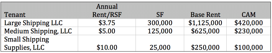
Your broker follows up his message with an email detailing the center’s numbers:
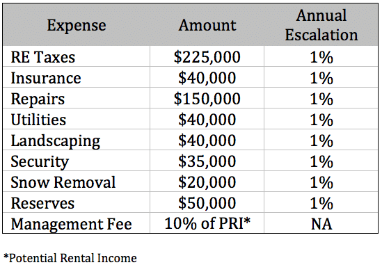
The projected operating expenses are as follows, and except for the reserves, all are reimbursable from the tenants on a pro-rata basis as CAM charges.
Before we start building the pro forma, we’ll need a few more assumptions:
Vacancy and Credit Loss
While all three tenants have been in the space for an extended period, are established businesses, and there are no indications of a downturn in the shipping industry, a 5% credit loss is assumed in an abundance of caution.
Potential Rental Income
Each tenant has negotiated flat rates through their lease terms (each of which extend beyond this five-year analysis), so base rent will remain constant. Additional rent, meaning the CAM charges, will inflate along with the projected expenses at 1% annually.
Financing
A quick call to the banker you’ve done business with for many years gave you all the information you need for the analysis: the lending market will likely support a loan for the intermodal center purchase: (i) on the lesser of a 1.30x debt service coverage ratio or 75% loan to value, (ii) at a 6% interest rate, and (iii) amortized over a 20-year term.
Sales Price and Cost of Sale
In that first phone call, your broker shared the not-yet-made-public sales price: $21,825,000. Assuming annual increases of 3%, you’ve projected you’ll be able to sell the property for $25,300,000 following the 5-year holding period. Additionally, you anticipate 3% in broker commissions and transaction costs on both your purchase and the sale.
Discount Rate
Considering your portfolio, and your investor’s expectations, you determine that the discount rate, your required rate of return, is 12%.
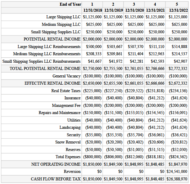
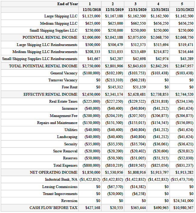
Industrial Investment Pro Forma
With the information provided by your broker, your banker, and your own return needs, you can now build a pro forma. While many folks rely on Excel spreadsheets to figure out the financials of a commercial real estate deal, rebuilding the sheets to reflect the uniqueness of each transaction, you can create the pro forma below, and all of the analyses following it, in just a few minutes with PropertyMetrics.
Next, using the above income stream and your banker’s direction that he’d loan up to the lesser of 1.30x DSCR or 75% LTV, you’ll need to figure out the maximum amount he’ll lend. Here it is:
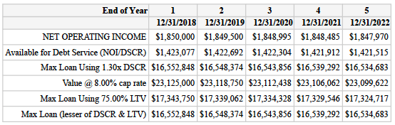
Okay, the maximum loan analysis shows that the maximum amount you can borrow, based on the Year 1 NOI in your pro forma is about $16,550,000. Plugging in that loan amount, and amortized over 20 years as suggested by your banker, your pro forma including debt service looks like this:
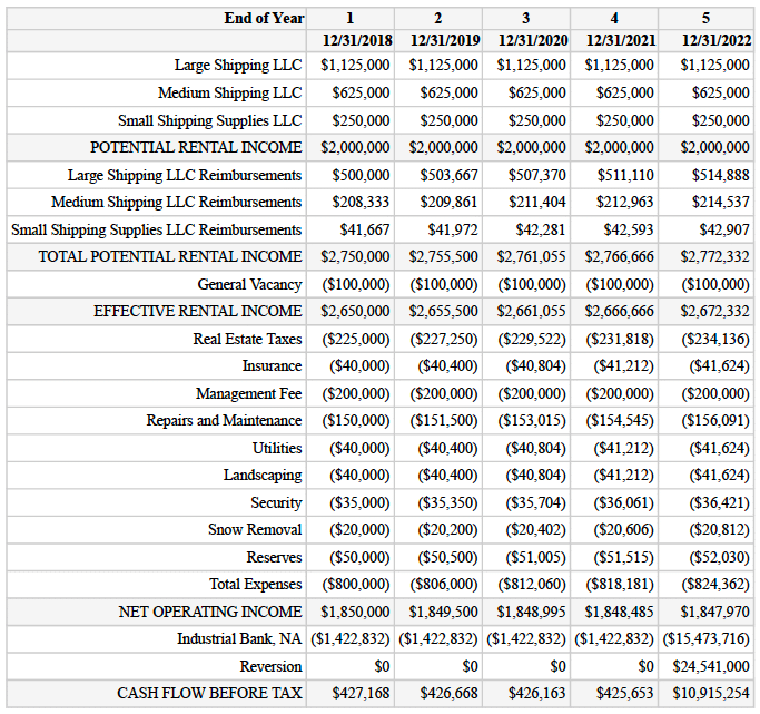
Yes, making debt service payments reduces cash in your pocket, however, as I’m sure you know, using the bank’s money instead of your own (i.e., reducing your equity requirement) is going to improve your yield.
Let’s dig a little deeper into this analysis with a few relevant financial ratios:
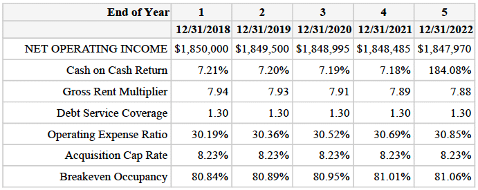
While the cash on cash seems troubling (your investors will be expecting returns of at least 12%), the IRR and NPV calculations (which consider the entire holding period) are a more relevant indication of return than cash on cash (which considers only a single year).
The next ratio, gross rent multiplier, is 7.94x in Year 1. As we’ve discussed in other articles, without context the GRM has little value, but when compared with the GRMs of comparable properties, it can reveal an anomaly. And if your GRM is drastically different than the comps, ask your broker to figure out why.
Impressively, our DSCR has hit our banker’s 1.30x requirement exactly. Although… that means there is virtually no wiggle room in your income. For example, if your vacancy creeps above your 5% assumption, and rental income drops, that 1.30x will be violated. We’ll take a look at a vacancy stress-test below.
The breakeven occupancy is about 81%, meaning vacancy/credit loss can increase from our projected 5% (already overly conservative given the history of the tenants) to just under 20% and still generate sufficient base and additional rent to cover expenses and debt service.
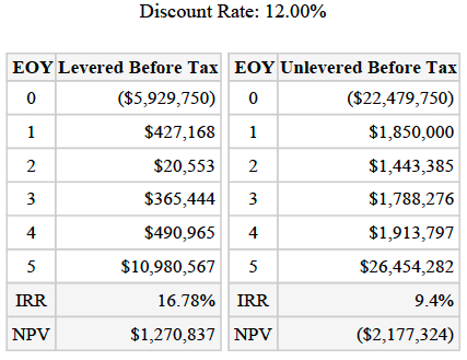
Industrial Discounted Cash Flow Analysis
On to the truly insightful numbers: your discounted cash flow analysis to determine IRR and NPV:
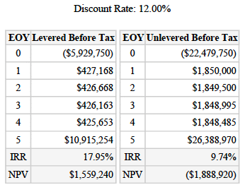
Now this looks better than the cash on cash. Your investors will be happy with an IRR of 17.95%, and even happier when you explain that the NPV number means they can pay $1,559, 240 over the current asking price and still get the 12% return they’re seeking.
Of course, it may also raise a few questions, like: (i) is a 12% return unreasonably low? and (ii) if it’s not, then why is this property almost 7% below what a comparable investor (one who can borrow on about the same terms as you) would offer? Let’s just say it might be a good idea to have a robust environmental review contingency included in your purchase contract.
Industrial Investment Vacancy/Credit Loss Sensitivity
Unless our assumptions were far off, or there are 38 undisclosed underground storage tanks buried behind the building, this deal seems worth a serious look. But it’s always a good idea to check worst-case scenarios. There are only three tenants in this property. What happens if the second largest, representing approximately 30% of center’s income disappears? It’s unlikely the space would go unfilled for five years, but let’s see what a 15% vacancy/credit loss rate would do our investor’s IRR.

15.18% return with a 15% vacancy credit loss over five years? You’ll take that every day, and twice on Sundays.
One more thought. As we mentioned above, any increase in vacancy above the assumed 5% is going to reduce property income to the point the bank’s 1.30x debt service requirement can’t be met. Let’s see what happens to the property’s DSC if we step up vacancy rates in 1% increments to 10%:

A single percentage point increase in vacancy rate to 6% and you’ve dropped to a 1.25x DSCR. Ordinarily this would be disconcerting, but given the history of the three tenants, the projected positive future of their shipping industry, and your determination that the 5% vacancy rate was overly cautious, perhaps the best takeaway from this sensitivity test is this: project a lower, more realistic vacancy rate, or risk the bank concluding there is a reasonable chance you can’t meet a 1.30x DSCR.
Leasing Market Assumptions
Okay, one last test. What if Medium Shipping, LLC’s term was set to expire at the end of Year 2? And Large Shipping, LLC could leave after Year 1? What happens if they both leave? What if only one of them renews?
What impact could these different outcomes have on your IRR projections? How do you explain likely returns to investors based on outcomes you can’t control? A market leasing assumptions analysis can help.
As discussed in this PropertyMetric’s article, in this type of analysis:
- One set of assumptions is used if a new tenant needs to be found
- The second set of assumptions is used if an existing tenant renews its lease, and
- There is a renewal probability that creates a weighted average between these two sets of assumptions.
Let’s run a market leasing assumptions analysis with the following assumptions:
Large Shipping, LLC – Lease expires 12/31/18
If they renew:
- Rent stays at current $3.75/RSF
- No commissions are incurred
- No rent abatement is required
- No tenant improvement allowance is granted
- There will be no period of vacancy
- The renewal term will be for four years, and
- There is a 50% chance they will renew
If they leave, and a new tenant comes in:
- Rent increases to $4.00/RSF market rate
- A 3% leasing commission is incurred
- 3 months of rent abatement is required
- A $40,000 TIA was negotiated
- The space is empty for three months, and
- The new term is also for four years.
Medium Shipping, LLC – Lease expires 12/31/19
If they renew:
- Rent stays at current $5.00/RSF
- No commissions are incurred
- No rent abatement is required
- MSLLC negotiates $10,000 in TIA
- The renewal term will be for three years, and
- There is a 75% chance they will renew
If they leave, and a new tenant comes in:
- Rent increases to $6.00/RSF market rate
- A 3% leasing commission is incurred
- Three months of abated rent is required
- The space is vacant for three months
- New tenant negotiates $25,000 in TIA, and
- The new term is also three years
Small Shipping Supplies, LLC – Lease expires 12/31/20
Because we’ll assume there is a 100% likelihood SSSLLC will renew, it’s not necessary to consider the new tenant/market assumptions. There is a 0% chance they’ll occur, so they’re not blended with the renewal assumptions.
Rent stays at $10.00/RSF, no commissions, no abatement, no TIA, no rent escalation, no vacancy period.
Here’s what the blended rates and expenses look like for each space:
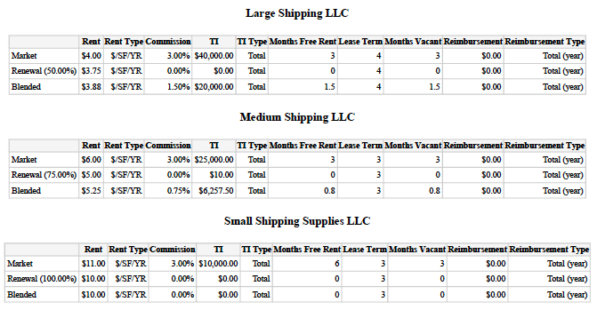
As you can see, the probability of renewal is what drives the blended rate. Because there is a 100% chance SSSLLC will stay and none of their terms will change, the market leasing assumptions aren’t blended with the renewal assumptions. The “blended” assumptions are simply equal to the renewal assumptions. Whereas with Large Shipping, LLC, because there is a 50% chance they’ll stay, the analysis gives a blended rate of the average of the market and renewal assumptions. And in Medium Shipping, LLC, when that is a 75% chance they’ll renew, the renewal assumptions are weighted more heavily than the market assumptions.
These blended assumptions can then be included in your pro forma to see the impact on your predicted cash flow….
And your IRR in a discounted cash flow analysis…
Conclusion
This case study illustrates one way to attack the financial analysis of a potential industrial property acquisition: (1) use your income and expense assumptions to determine how much you can borrow; (2) take a look at the financial ratios we considered above; (3) determine the projected return; and (4) stress-test your model for variables like vacancy rate. And, where leases will be expiring during your holding period, your investors can gain some comfort by seeing a lease market assumptions analysis to understand a predicted IRRs based on the likelihood of renewals vs. new leases.
Now, I don’t know about you, but I’m pulling the trigger on this deal. That is, at least until my Phase II unearths those storage tanks…
If you have any comments or questions, please leave them in the section below!