
An investor is considering Oakview Industrial Center, a fully leased industrial property with an asking price of $4.75 million. All three tenant leases expire during his planned five-year holding period. He has asked us to underwrite the acquisition and help him determine what he can afford to offer.
His plan is to renew the existing leases where possible, find new tenants for any vacant space, and sell with several years remaining on the new leases. He intends to pursue renewals, but doesn’t want the purchase to depend on getting them. He has asked us to test what happens if all three tenants leave and each suite takes six months to lease again.
The investor’s target is a 12% pretax equity internal rate of return, or IRR. We need to determine what purchase price meets that requirement under the stated re-leasing assumptions.
We’ll work through the analysis in PropertyMetrics Proforma, starting with the income from the existing leases and building toward the investment return.
The property and its existing leases
Oakview contains 30,000 rentable square feet in Central Florida, divided into three comparable warehouse suites with modest office buildouts. We assume the investor acquires the property on January 1, 2027 and sells on December 31, 2031. The business plan allows for routine upkeep and limited work to prepare suites for tenants, but no major redevelopment.
The starting point is the rent roll and the terms of each existing lease. In the table below, base rent is shown at the original lease commencement date, in annual dollars per square foot, with payments made monthly. We enter that starting rent together with the lease’s escalation schedule so the model can determine the rent due during our projection.
Existing leases and rent increases
| Tenant | Area | Original base rent | Lease commencement | Lease expiration |
|---|---|---|---|---|
| A: Distribution | 10,000 SF | $11.00/SF/year | July 1, 2025 | June 30, 2029 |
| B: Packaging | 10,000 SF | $12.00/SF/year | April 1, 2026 | March 31, 2030 |
| C: Industrial supplies | 10,000 SF | $13.00/SF/year | January 1, 2026 | December 31, 2028 |
The rent increases under those leases are as follows:
| Tenant | Rent increase | Effective dates within the existing lease |
|---|---|---|
| A | 3% of previous rent every 12 months | July 1, 2026; July 1, 2027; July 1, 2028 |
| B | Add $0.50/SF to the annual rate every 18 months | October 1, 2027; April 1, 2029 |
| C | None | Flat through December 31, 2028 |
Tenant A has already received one increase before the acquisition. Tenant B’s next increase takes effect in October 2027, nine months into the first projection year. Its annual income will therefore include nine months at $12.00 per square foot and three months at $12.50:
10,000 SF × [($12.00 × 9/12) + ($12.50 × 3/12)] = $121,250
Applying all three schedules produces approximately $366,250 of base rent in 2027. We assume there are no early-termination rights, fixed-price renewal options, or outstanding original tenant-improvement and commission obligations that change this forecast.
Base rent is only part of the property’s income. The leases also require tenants to reimburse certain operating expenses, so our next step is to work through the expense budget and determine how much of it the owner can recover.
Operating expenses and tenant reimbursements
We use the following operating budget for the first year of ownership:
| Expense | 2027 annual budget | Fixed % |
|---|---|---|
| Property taxes | $75,000 | 100% |
| Property insurance | $24,000 | 100% |
| Common-area maintenance (CAM) | $45,000 | 100% |
| Property management | $18,000 | 100% |
| Total | $162,000 |
We enter these expenses as 100% fixed with respect to occupancy because the budgets do not decrease when a suite becomes vacant. Management is a flat retainer, and tenants pay separately metered suite utilities directly. We spread building expenses evenly by month.
Property taxes, insurance, and CAM total $144,000 in the first year. Under their existing leases, A and B each reimburse one-third of those expenses, or $48,000. The owner is responsible for the management fee, which is excluded from every tenant’s reimbursements.
C reimburses the same proportion of taxes and insurance, but its CAM obligation is subject to a fixed $1.00/SF annual expense stop. The CAM budget works out to $1.50/SF across the building. C pays the $0.50/SF above the stop, or $5,000 for its suite, while the owner pays the remaining $10,000 of C’s CAM share. Including taxes and insurance, C’s total reimbursement is $38,000.
Total tenant reimbursements are therefore $134,000. Adding them to base rent gives approximately $500,250 of gross income. After deducting the 1% General Vacancy allowance and the operating expenses, we arrive at net operating income, or NOI, for the first year:
| First-year income calculation | Amount |
|---|---|
| Base rent | $366,250 |
| Tenant reimbursements | $134,000 |
| Gross income | $500,250 |
| General Vacancy allowance | ($5,002) |
| Operating expenses | ($162,000) |
| Net operating income | $333,247 |
Displayed amounts are rounded from the monthly calculations, so adding rounded lines may differ from a displayed total by $1.
The 1% general vacancy allowance is a case assumption, not a measured market vacancy rate or a separate credit-loss estimate. We’ll model the specific lease vacancies later. Reimbursements retain each suite’s one-third share of the whole building, so occupied tenants do not pick up a vacant suite’s costs.
The resulting NOI gives us a starting point for the acquisition analysis. It shows what the existing leases produce after operating expenses, before financing and capital expenditures. Before extending the forecast through the lease expirations, we need to establish how the expense budgets and future leasing estimates change over time.
Inflation assumptions
We use January 1, 2027 as the base date for the operating expense budgets, recurring replacement allowance, and estimates of market rent and tenant improvements (TI). The inflation profiles specify the annual change applied to each of those inputs:
| Inflation profile | Annual rate | Applied to |
|---|---|---|
| Market Inflation | 0% | Market and renewal starting rents before the next lease begins |
| Expense Inflation | 3% | Property taxes, insurance, CAM, management, the recurring replacement allowance, and both renewal and new-tenant TI allowances |
| General Inflation | 0% | No additional growth assigned in this case |
The first Expense Inflation adjustment occurs on January 1, 2028, with another 3% increase each January 1 thereafter. Expenses and TI allowances for 2029 therefore reflect two years of compounded increases from the 2027 estimates.
With Market Inflation at 0%, we hold market and renewal starting rents at their January 2027 levels until the next lease begins. The acquisition therefore does not rely on market-wide rent growth, although market rents could still decline. Rent increases within a lease are separate: the existing contracts retain their stated schedules, and the future leases described below have their own 3% annual increases beginning on the first lease anniversary. Those contractual increases are not an application of Expense Inflation.
Underwriting the next round of leases
We’ll start with the renewal case. The investor seeks a new seven-year term for each tenant, beginning immediately after its existing lease expires. We assume a starting annual rent of $13.00 per square foot for all three suites, with 3% increases on each anniversary of the new lease.
Each new lease also requires full one-third reimbursement of taxes, insurance, and CAM, with management excluded. For C, this means negotiating away the CAM stop after its current lease expires on December 31, 2028. Its starting base rent remains $13.00/SF, but its total occupancy cost increases as it assumes expenses previously paid by the owner.
The same starting rent and expense-recovery structure apply if the investor must find a new tenant. What changes is the downtime and the cost of securing the lease. We enter both sets of market leasing assumptions now, even though we will first run the model with all tenants renewing:
| Input, per suite | Market / replacement tenant | Renewal |
|---|---|---|
| Starting annual base rent | $13.00/SF | $13.00/SF |
| Tenant-improvement (TI) allowance, in January 2027 dollars | $80,000 | $20,000 |
| Leasing commission | 5% | 2% |
| Free rent after commencement | 0 months | 0 months |
| Months vacant | 6 months | 0 months |
In PMX, the seven-year term, 3% annual rent increases, and future reimbursements are shared non-weighted assumptions. They apply whether the existing tenant renews or a new tenant takes the space, with rent increases beginning after the first twelve months.
We set the renewal probability to 100% for each tenant in this first projection. This selects the renewal rent and costs without downtime. The replacement tenant market assumptions with six-month market downtime remain in the inputs for the later comparison.
The tenant-improvement (TI) allowances cover limited work in space that can be reused. Using the January 2027 estimates and the 3% Expense Inflation profile above, C’s January 2029 renewal TI allowance includes two annual increases: $20,000 × 1.03², or $21,218.
Leasing commissions are calculated on the full seven years of base rent, including the annual increases, but not on reimbursements. That means the owner pays a commission for the entire lease even though he plans to sell before it expires. We assume the improvement allowance and commission are paid when the new term begins. The terms and payment dates are assumptions for the analysis and would need to be confirmed during leasing negotiations.
Separately, we budget a $9,000 annual replacement allowance for recurring capital expenditures in 2027. It increases 3% through Expense Inflation and is spread evenly by month. We deduct this spending below NOI, without tenant reimbursement, and keep it separate from tenant improvements and commissions.
Property cash flow before debt service
C’s renewal begins in January 2029, A’s in July 2029, and B’s in April 2030. There is no loss of rent between leases, but the owner spends approximately $124,000 on improvements and commissions to obtain those commitments. Here is the full proforma before debt at this point:
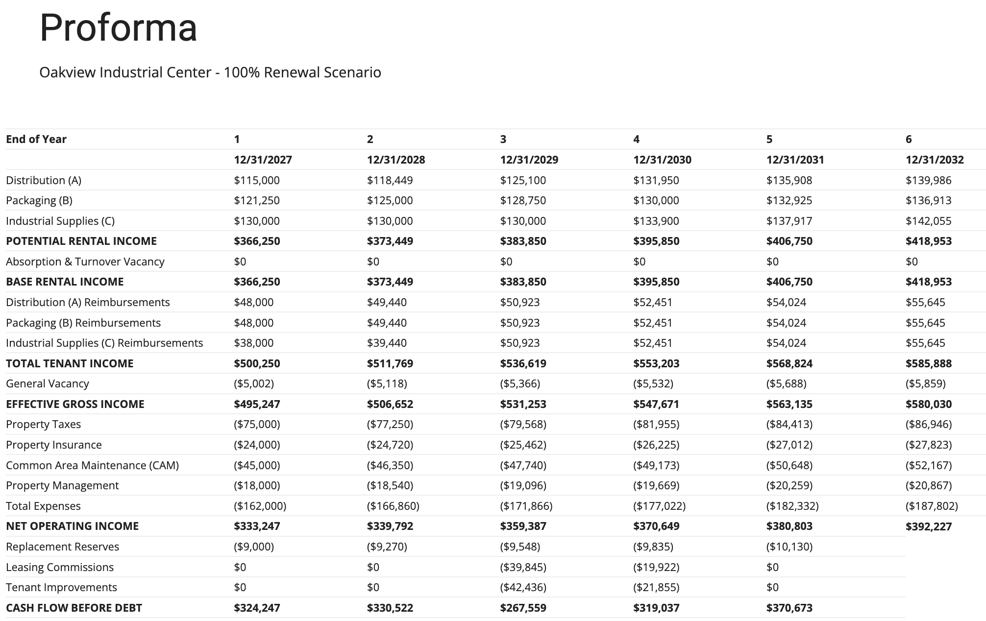
After all costs and the annual replacement allowance, cash flow before debt service and sale proceeds is:
| Renewal scenario | 2027 | 2028 | 2029 | 2030 | 2031 |
|---|---|---|---|---|---|
| Cash flow before debt | $324,247 | $330,522 | $267,559 | $319,037 | $370,673 |
The decline in 2029 reflects the cost of renewing C and A in the same year. B’s renewal costs follow in 2030. Occupancy remains at 100%, but the amount available to pay debt service and distribute to the investor falls during the leasing years. Those costs need to be included even in the outcome where the retention effort succeeds.
We now have a property-level forecast that includes both the operating income and the cost of the leasing plan. The next step is to add the acquisition financing and determine how much cash the investor must contribute at closing and can expect to receive during ownership.
Sizing the acquisition loan
For the financing, we assume a fixed 6% interest rate, monthly payments based on 25-year amortization, and a five-year loan term. The remaining principal balance is due at maturity. The proposed lender limits the loan to 65% loan-to-value and requires a minimum 1.30x debt service coverage ratio, or DSCR, for initial sizing.
For this example, the lender’s coverage calculation uses first-year NOI after deducting the replacement allowance. We assume the lender accepts our operating forecast for this initial test and a property value equal to the purchase price. We therefore calculate one loan limit from 65% of the price and another from the available income, then select the lower amount.
First-year NOI of $333,247, less the $9,000 replacement allowance, leaves $324,247 for the coverage test. A 1.30x requirement means that income must equal at least $1.30 for each dollar of scheduled principal and interest. Dividing by 1.30 gives the maximum annual debt service:
$324,247 ÷ 1.30 ≈ $249,421 of maximum annual debt service
At the assumed 6% rate and 25-year monthly amortization, that annual payment supports a loan of approximately $3,225,985. The price-based limit is lower: 65% of the $4.75 million asking price is $3,087,500. We use that amount as the acquisition loan.
The resulting annual debt service is $238,714, giving first-year coverage of 1.36x after the replacement allowance. Subtracting those payments from the property’s cash flow leaves the following amount for equity:
$324,247 − $238,714 = $85,533
The loan also carries a 1% origination fee, or $30,875. In addition, the buyer has budgeted $135,000 for other acquisition costs. Adding the purchase price, those costs, and the loan fee, then subtracting the loan proceeds, gives an initial equity investment of $1,828,375. This is the cash required for the acquisition, not the total capital that may be needed during ownership. The loan has no additional advances to cover future leasing costs.
This establishes the borrowing assumed in our model, but does not complete the lender’s underwriting. The lender must also review the lease expirations and the investor’s ability to fund vacancy, which becomes important in the non-renewal case. First, we’ll complete the renewal analysis by adding the sale proceeds.
Estimating sale proceeds and the equity return
With the assumed seven-year renewals, C’s lease runs through December 2035, A’s through June 2036, and B’s through March 2037. At the December 2031 sale, each has between four and just over five years remaining. The buyer receives a rent roll with this round of leasing completed and paid for, rather than expirations soon after acquisition.
To estimate the sale price, we capitalize the following year’s projected NOI at a 7.50% exit capitalization rate:
Gross sale price = 2032 property NOI ÷ 7.50%
The renewal forecast produces approximately $392,227 of NOI in 2032, before the replacement allowance. Capitalizing that income gives the estimated gross sale price. We then deduct 3% selling costs and the loan balance remaining after the final scheduled payment:
| Renewal-case sale at December 31, 2031 | Amount |
|---|---|
| Gross sale price | $5,229,696 |
| Selling costs at 3% | ($156,891) |
| Loan balance after the final scheduled payment | ($2,776,653) |
| Net sale proceeds to equity | $2,296,152 |
The exit cap applies to NOI before the recurring replacement allowance, while lender coverage uses income after that allowance. We project 2032 to estimate what the next buyer would pay for the income stream. Our investor sells at the end of 2031 and does not receive that following year’s operating cash flow.
One note about the property taxes after the sale. Instead of trying to estimate a reassessment following the sale, we just use our 3% annual inflation again in the year after the sale. Since all three leases will fully reimburse property taxes, there would only be a small net effect from the 1% general vacancy allowance. Later we’ll also test a range of exit cap rates.
The 7.50% exit cap remains an assumption, not a rate established by comparable sales for this hypothetical property. Longer lease terms give the buyer more visibility into the income, but tenant credit, building condition, and eventual re-leasing costs still matter. The contractual increases also put the later rents above our assumed flat market rent. We will also test an 8.00% exit cap, and then examine a wider range of sale outcomes and refinancing before deciding whether to proceed at the proposed price. Here’s our complete proforma at this point:
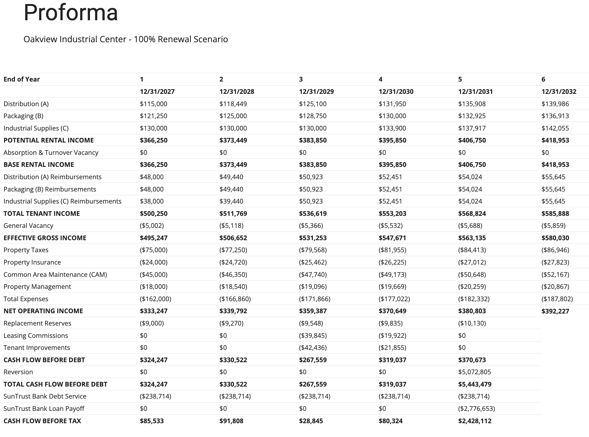
The renewal proforma includes the existing leases, renewal costs, operating expenses, debt service, and net sale proceeds at the end of 2031.
We can now calculate the investor’s return using the initial equity investment, the cash flows during ownership, and the net sale proceeds. XIRR on the dated monthly equity cash flows gives an annualized return of 8.94%. The property generates cash flow and the leasing plan is completed, but the return is still below the investor’s 12% requirement at the asking price.
Every return calculation uses the same dated monthly convention. Positive cash flow is treated as a distribution and a shortfall as an additional contribution. The annual proformas summarize those amounts, while XIRR retains their timing.
We also calculate the equity multiple, which divides total distributions by all equity contributed. It shows how much cash comes back for each dollar invested, including the return of that dollar. Unlike XIRR, it does not account for when the money is received. Both measures use the same equity cash-flow schedule, including any additional contributions during ownership.
Equity multiple = total equity distributions ÷ total equity contributions
In the renewal case at the $4.75 million asking price, the investor contributes $1,828,375 at acquisition. Under our assumption that monthly surpluses are distributed, he also contributes approximately $95,729 during months when renewal expenditures exceed the available property cash flow. Although each year’s net cash flow is positive, those individual months still require funding.
Total equity contributions are therefore approximately $1,924,104. Over the five-year holding period, the investor receives approximately $2,810,351 in distributions, including the sale proceeds after selling costs and loan repayment. The equity multiple is:
Equity multiple = $2,810,351 ÷ $1,924,104 ≈ 1.46x
The investor receives approximately $1.46 for every dollar contributed, including the return of his capital. The multiple describes the total cash returned, while the 8.94% XIRR accounts for when he contributes and receives that money. Both measures use the same monthly equity cash flows.
The renewal case therefore produces a profit, but its 8.94% annualized return remains below the investor’s 12% requirement. Before deciding how much less to offer, we need to examine the cost of finding new tenants, which is the outcome he has asked us to use in setting his price limit.
If the tenants do not renew
We keep the purchase price and acquisition loan unchanged, then set every tenant’s renewal probability to 0%. The model now uses the new-tenant improvement allowances and commissions, together with the six-month downtime assumption. The existing leases still expire on their original dates:
| Suite | Vacancy period | Replacement lease begins |
|---|---|---|
| C | January–June 2029 | July 1, 2029 |
| A | July–December 2029 | January 1, 2030 |
| B | April–September 2030 | October 1, 2030 |
C’s new tenant starts paying rent just as A vacates. Although each suite takes six months to lease, the two vacancies occur back to back, leaving one-third of the building empty throughout 2029. At the assumed $13.00/SF starting rent, those periods of vacancy remove $130,000 of base rent:
2 suites × 10,000 SF × $13.00/SF/year × 6/12 = $130,000
The loss extends beyond base rent. The owner also receives no expense reimbursements from a vacant suite, while the property taxes, insurance, CAM, management fee, and loan payments continue. B’s departure creates another six-month vacancy in 2030 and another $65,000 of lost base rent. In the displayed projection, these turnover losses are large enough that there is no separate General Vacancy deduction in either year.
The new leases also require cash before they have generated much income for the owner. Under our payment assumptions, C’s improvement allowance and commission are paid in July 2029, A’s in January 2030, and B’s in October 2030. Reviewing the monthly projection lets us see those expenditures alongside the income coming in from the other suites.
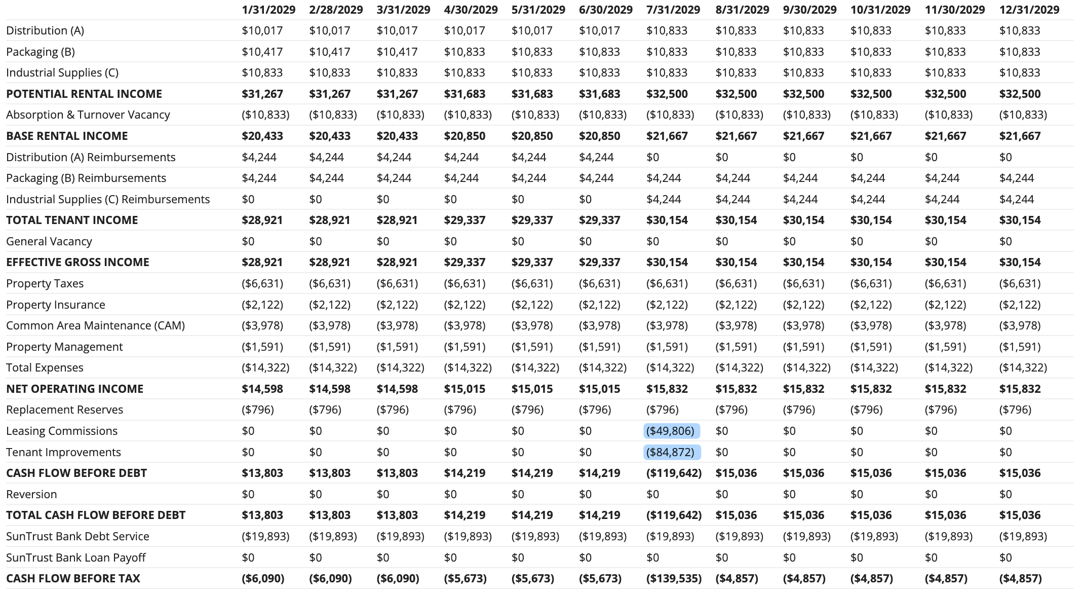
Monthly cash flow for the non-renewal case in 2029.
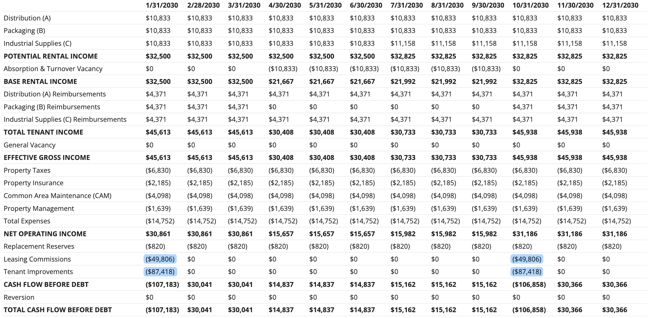
The 2030 projection shows A’s January leasing costs, B’s vacancy and October leasing costs, and the return to full occupancy.
Total tenant improvements and leasing commissions increase from approximately $124,000 in the renewal case to $409,000 when every suite must be re-leased. Combined with the lost rent and reimbursements, that additional spending produces a very different cash-flow pattern:
| Measure at the $4.75 million asking price | All tenants renew | No tenants renew |
|---|---|---|
| 2029 equity cash flow | $28,845 | ($199,109) |
| 2030 equity cash flow | $80,324 | ($241,941) |
| Total improvements and commissions | $124,058 | $409,126 |
The negative cash flows in 2029 and 2030 show that the equity required at closing is not the investor’s entire funding obligation. He also needs enough available capital to carry the property through the leasing period. The annual totals show the size of each year’s deficit, while the monthly projection identifies when contributions will be needed.
For the return calculation, we continue to treat those monthly deficits as additional equity contributions and have not assumed a leasing reserve funded at acquisition. The investor could retain earlier cash flow or set aside funds at closing, but either approach changes when money is invested and distributed.
Debt coverage is another concern. The non-renewal case falls to 0.73x lender-adjusted DSCR in 2029, so income after the replacement allowance does not cover scheduled loan payments, even before tenant improvements and commissions. It is not automatically a covenant breach, since our 1.30x initial sizing assumption does not define an ongoing loan covenant. However, a lender would need to address that projected shortfall in its underwriting.
Here is the completed proforma for the non-renewal scenario:
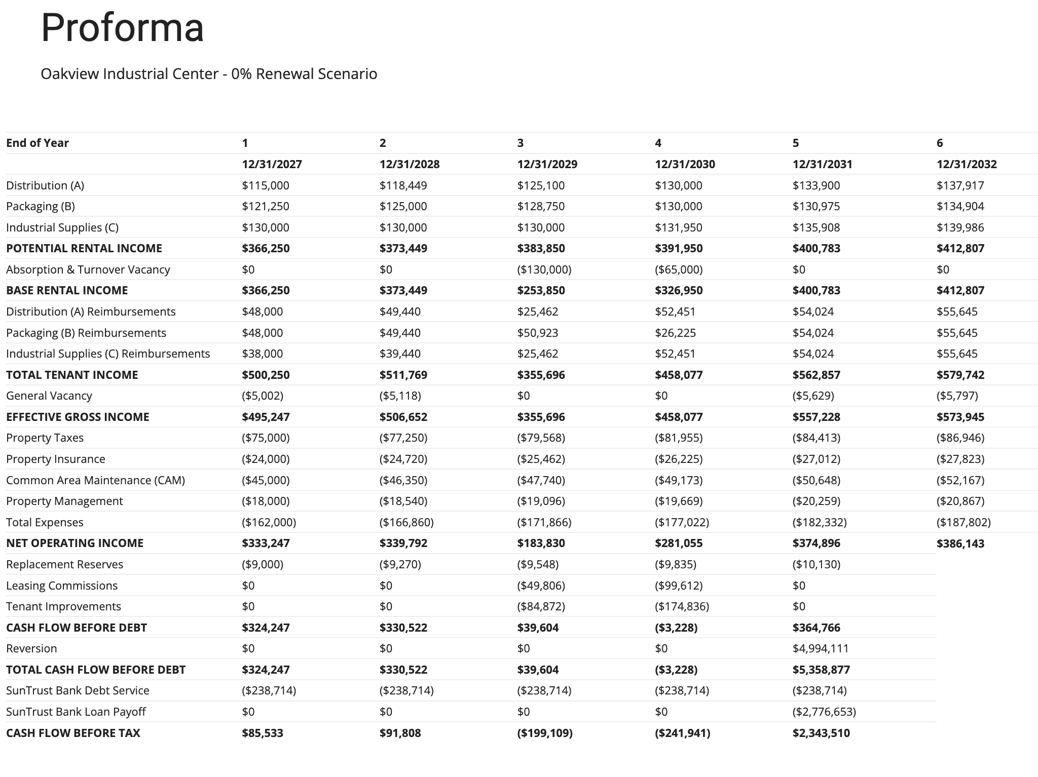
The non-renewal proforma includes the income lost during vacancy, the cost of re-leasing all three suites, acquisition debt, and the eventual sale.
All three new tenants are paying by October 1, 2030, leaving fifteen full months of collections before sale. Their leases expire between June 2036 and September 2037. The later commencement dates also shift the rent increases and change the 2032 NOI. We use that revised income to calculate this case’s sale proceeds, retaining the same 7.50% exit cap.
At the asking price, the non-renewal case produces an annualized equity return of 2.59%. The investor still reaches the same broad objective of selling a fully leased property with several years remaining on the leases. However, the income lost during vacancy and the higher leasing costs leave far less return on the capital required. We can now test what purchase price would make that plan acceptable to this investor.
Testing lower purchase prices
We test purchase prices of $4.35 million and $4.00 million alongside the seller’s asking price. The rent forecasts, expense budgets, and leasing assumptions remain unchanged. A lower purchase price does change the financing, so we recalculate the acquisition loan, origination fee, initial equity, debt service, and loan payoff at each proposed price.
| Purchase price | 65% price limit | 1.30x adjusted DSCR limit | Loan used |
|---|---|---|---|
| $4,750,000 | $3,087,500 | $3,225,985 | $3,087,500 |
| $4,350,000 | $2,827,500 | $3,225,985 | $2,827,500 |
| $4,000,000 | $2,600,000 | $3,225,985 | $2,600,000 |
The income-based limit stays unchanged because first-year income, the interest rate, and amortization are unchanged. The 65% purchase-price limit is lower at every tested price and therefore determines borrowing. At any given price, both leasing scenarios retain the same acquisition loan. We do not reduce the original debt merely because a tenant leaves.
We also retain the buyer’s $75,000 first-year property-tax estimate, increasing 3% annually, and the $135,000 allowance for other acquisition costs. The lower offers receive no credit for possible savings in those budgets. The tax estimate and closing costs would still need to be confirmed before proceeding, while the origination fee changes with the loan in each run.
After updating the financing at each price, we obtain the following returns:
| Purchase price | Equity XIRR: all renew | Equity XIRR: none renew |
|---|---|---|
| $4,750,000 | 8.94% | 2.59% |
| $4,350,000 | 13.96% | 7.58% |
| $4,000,000 | 18.58% | 12.13% |
At $4.35 million, the renewal case meets the investor’s target, but the non-renewal case does not. Paying that amount would mean accepting a lower return if all three tenants leave. At $4.00 million, the non-renewal case reaches 12.13%, which meets the requirement the investor gave us under the stated leasing, financing, and sale assumptions.
We can narrow the price range further by adjusting the purchase price and loan amount until the monthly equity cash flows produce a 12% return. We repeat that calculation at an 8.00% exit cap to see how a lower resale value changes the result. The approximate price limits below are rounded to the nearest $1,000:
| Exit cap | Price limit: all renew | Price limit: none renew |
|---|---|---|
| 7.50% | $4,504,000 | $4,010,000 |
| 8.00% | $4,299,000 | $3,809,000 |
At the 7.50% base exit cap, the non-renewal case supports approximately $4.01 million. At 8.00%, that falls to about $3.81 million. Although the leasing plan is completed in both cases, the higher cap reduces sale proceeds. At unchanged income, moving from 7.50% to 8.00% lowers gross sale value by 6.25%, materially affecting what the investor can pay today.
The investor’s stated requirement is 12% in the non-renewal case at the 7.50% base exit cap. The 8.00% case is an additional sensitivity for him to consider, not a second return requirement. These calculations show what the property is worth to this investor under the specified assumptions. They do not establish market value or tell him what the seller will accept.
The equity required at a $4 million purchase
The return comparison points us toward a $4 million offer, but the investor also needs to understand the amount of capital involved. We total the initial investment and every additional monthly contribution, then compare them with all distributions from operations and the sale. These figures use the same monthly cash-flow convention as XIRR and the 7.50% base exit cap.
| At a $4 million purchase | All tenants renew | No tenants renew |
|---|---|---|
| Initial equity at acquisition | $1,561,000 | $1,561,000 |
| Additional equity contributed during ownership | $86,306 | $419,475 |
| Total equity contributed | $1,647,306 | $1,980,475 |
| Total distributions, including net sale proceeds | $3,427,805 | $3,126,154 |
| Projected profit before income taxes | $1,780,499 | $1,145,679 |
| Equity XIRR | 18.58% | 12.13% |
| Equity multiple | 2.08x | 1.58x |
In the non-renewal case, the investor contributes approximately $1.98 million in total, including about $419,000 after acquisition, and receives approximately $3.13 million. The resulting profit is about $1.15 million before income taxes. The 1.58x equity multiple means approximately $1.58 is returned for every dollar contributed over the investment. It is not a 58% annual return.
The renewal case also includes later contributions, even though its annual cash flows are positive. Under our distribution assumption, earlier monthly surpluses have already been paid out when a renewal bill creates a shortfall. We therefore calculate contributions and distributions from the monthly schedule, rather than netting the year’s positive and negative months together first.
Dividing distributions only by the $1,561,000 contributed at acquisition would omit the later capital calls and overstate the multiple. The contribution totals are not a recommendation to deposit that amount in a reserve at closing. Retaining cash, prefunding a reserve, or adding sponsor fees would change the investor cash flows and require recalculating both measures. This case models the property owner’s equity before income taxes, without a separate sponsor fee or partnership waterfall.
The investor has not specified a minimum equity multiple in addition to the 12% return target. We use it to explain the capital commitment and payoff, not to introduce another hurdle after seeing the result.
Testing a weaker sale market
The price-limit table shows how much less the investor could pay to preserve a 12% return at a higher exit cap. We now examine the property he would actually own at a $4 million purchase price. Using the non-renewal scenario, we change only the exit cap and retain the $2.60 million acquisition loan, the leasing timetable, and the operating forecast.
The projected 2032 NOI is approximately $386,143 before the replacement allowance. Capitalizing that income at each rate produces the following gross sale values. Note that we use the unrounded NOI to calculate each gross sale price, then round the results for presentation. The returns and multiples also include the 3% selling costs, repayment of the original loan, and all the preceding equity cash flows:
| Exit cap | Gross sale price | Equity XIRR | Equity multiple |
|---|---|---|---|
| 7.50% (base) | $5,148,569 | 12.13% | 1.58x |
| 8.00% | $4,826,783 | 9.32% | 1.42x |
| 9.00% | $4,290,474 | 3.90% | 1.16x |
| 10.00% | $3,861,426 | -1.42% | 0.95x |
Calculations use unrounded amounts. Recalculating sale prices from the rounded NOI shown in the text may produce small differences.
At an 8.00% exit cap, the investor misses the target but still receives about $1.42 for every dollar contributed. At 9.00%, that falls to $1.16. The 10.00% case returns only about $0.95 per dollar, with total distributions approximately $103,000 below total contributions. The equity multiple makes the difference between a lower return and a nominal loss of capital easier to see.
The multiple does not make the sale estimate more certain. Its numerator contains the same projected sale proceeds used in XIRR. These tests hold income and leasing costs unchanged and are not a forecast or a worst-case boundary. A downturn that also lengthens vacancy, reduces rent collections, or requires more tenant work would affect the operating cash flows as well.
The investor must decide whether those potential outcomes are acceptable. He also needs to determine whether he could keep the property if selling in 2031 is unattractive, because the acquisition loan matures at the same time as the planned sale.
Refinancing instead of selling
Let’s do one more check on whether the investor could refinance the loan at the end of the loan term, should he not be able to sell the property. At the $4 million purchase price, the original $2.60 million loan has approximately $2,338,234 remaining after the final scheduled payment in 2031.
We test refinancing separately from the five-year sale analysis. There is no sale in this alternative, no 3% selling cost, and no refinancing distribution added to the sale XIRR or equity multiple. This is a check of available loan proceeds and the first year of payments, not a return calculation for a longer holding period.
Assume a new lender allows 60% loan-to-value, requires 1.30x coverage after the replacement allowance, and uses 25-year amortization with monthly payments. We test fixed interest rates of 8% and 10%. For value, we capitalize the applicable 2032 NOI before the allowance at 9.00%. These are hypothetical stress assumptions, not future loan commitments.
At each interest rate, we test the forecast NOI and a second case with NOI 25% lower. The reduced NOI is used for both valuation and coverage, while the full $10,433 replacement reserve allowance for 2032 remains in the coverage calculation. This is a sensitivity on sustainable income at refinancing. It does not automatically reduce signed contract rents or revise the first five years of operations.
We calculate the loans supported by value and income, then use the smaller limit. Because the investor takes no cash out and pays transaction costs separately, actual new borrowing is capped at the old loan balance. Any difference between that balance and the new loan must be paid from equity:
| Refinancing test | Maximum supported loan | New loan used | Principal paydown from equity* |
|---|---|---|---|
| Forecast NOI, 8% interest | $2,574,284 | $2,338,234 | $0 |
| Forecast NOI, 10% interest | $2,574,284 | $2,338,234 | $0 |
| NOI 25% lower, 8% interest | $1,930,713 | $1,930,713 | $407,521 |
| NOI 25% lower, 10% interest | $1,930,713 | $1,930,713 | $407,521 |
*The paydown excludes refinancing fees and additional required reserve or escrow deposits. Those amounts have not been specified and must be added to determine total cash needed at closing. A $0 paydown does not mean a cost-free refinancing.
The loan-to-value-based limit controls all four tests. With forecast NOI, it supports enough borrowing to repay the old loan. With NOI 25% lower, it supports only about $1.93 million, leaving a principal shortfall of approximately $408,000 before fees and reserves. The higher interest rate does not reduce proceeds in these particular rows because the LTV limit is already more restrictive, but it increases the new loan payments.
Using the actual new principal in each case, we calculate annual debt service and subtract it from NOI after the full replacement allowance:
| Refinancing test | Annual debt service | 2032 cash after allowance and debt |
|---|---|---|
| Forecast NOI, 8% interest | $216,562 | $159,147 |
| Forecast NOI, 10% interest | $254,971 | $120,739 |
| NOI 25% lower, 8% interest | $178,819 | $100,355 |
| NOI 25% lower, 10% interest | $210,533 | $68,641 |
The positive annual cash flows do not establish that the investor can fund the paydown. They also exclude closing cash and any additional leasing or capital costs beyond the recurring allowance. If a tenant default caused the lower income, for example, the cost of restoring occupancy would need to be modeled separately.
A refinancing loan would still depend on tenant credit, remaining lease terms, the lender’s valuation, and the borrower’s financial capacity. Any equity needed here would be additional to capital already contributed during the original leasing program. The investor should not count the same available funds as protection against both obligations. Refinancing may provide time to hold, but the ratio calculations alone do not establish that a loan will be available or that holding is preferable to selling.
The investor’s proposed offer
The investor uses $4.00 million as his proposed offer, subject to confirming the leasing, financing, and funding assumptions. At that price, the non-renewal case produces approximately a 12.1% annualized equity return and a 1.58x equity multiple at the 7.50% base exit cap. Under the modeled distribution policy, he contributes approximately $1.98 million in total and receives approximately $3.13 million through operations and the sale.
Successful renewals would improve the result, but the purchase does not depend on them to meet the stated base-case target. The roughly $10,000 between the offer and the modeled ceiling is not a substantial margin of safety. Before submitting the offer, the investor must decide whether the lower-return sale outcomes are acceptable and establish how he would fund the leasing period and any refinancing shortfall.
That review includes the evidence for seven-year leases at $13.00/SF, C’s change to full CAM recovery, the suite-improvement budgets, and the proposed loan terms. None is established merely because the model produces a 12% return. A smaller acquisition loan, a required reserve funded at closing, or more expensive leasing terms would require recalculating the offer rather than changing only the conclusion.
If the investor cannot accept the downside or make the necessary capital available, his choices include reducing the price, borrowing less, arranging different loan terms, or passing on the property. The seller may not accept $4 million. What the analysis provides is a financial basis for that decision, connecting the income being acquired, the cost of the leasing plan, the total equity commitment, and the possible outcomes at sale or loan maturity.