When working with a commercial real estate data set, there are occasions where it is necessary to create a sum for a range of values, but only if they meet certain criteria. Fortunately, there is an easy way to accomplish this task using a built in Microsoft Excel function known as “SUMIF.”
In this article, the SUMIF function is defined, the syntax for using it is described, and its use is demonstrated in a commercial real estate scenario.
What is the SUMIF Function?
SUMIF is a Microsoft Excel function that allows a user to sum a range of values, but only if a given set of criteria is met. With regard to CRE analysis, this function is particularly useful when performing financial analysis on data sets that have been provided by a broker or property owner.
SUMIF Syntax
Like every function in Excel, proper use of SUMIF requires the user to write the formula using a specific syntax. It is:
SUMIF Required Syntax: SUMIF(range, criteria, [sum_range])
In order to understand how this works, it is helpful to break the function into its components.
SUMIF is the name of the function. All uses of the SUMIF function will begin with an equal sign (=) followed by the function name. This is how Excel knows which function it is working with. This argument is required.
Range refers to the range of numeric values to be summed. For example, in commercial real estate, this could be the output from a rent roll or operating statement. This argument is required.
Criteria refers to the condition under which values should be summed. Depending on the context, these could be a number, cell reference, text, or another function. This argument is required,
Sum Range refers to the range of cells to be added, but only if it is different from the defined range. As such, this argument is optional.
To demonstrate how these arguments work, an example is helpful.
SUMIF Example
There are countless ways in which the SUMIF function can be used in real estate financial modeling, but one of the most common ones is described in the example below.
Suppose that a commercial real estate analyst has received a data export for a property on which they are performing due diligence. It includes a bank ledger with 1 month’s worth of line item expenses, a selection of which are shown in the worksheet below:
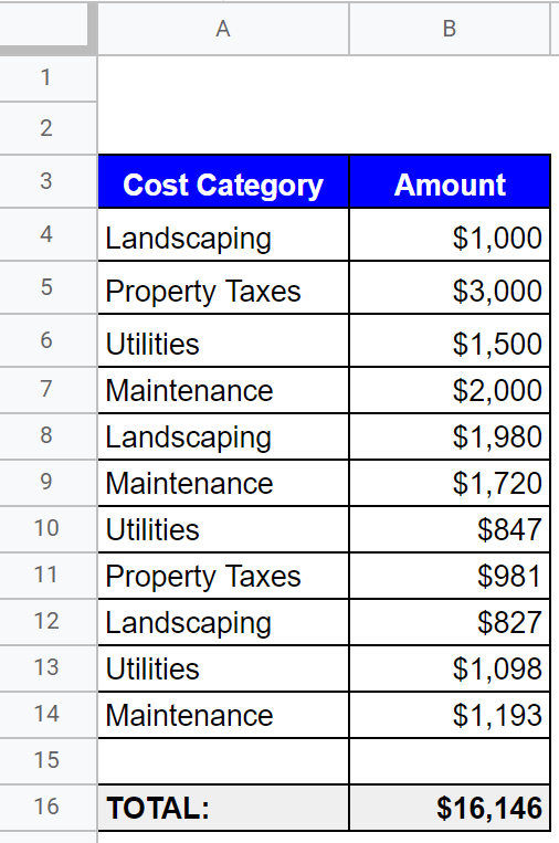
In column A of this table, a description of the expense category is provided. In column b, the amount is shown. The analyst’s job is to sum the costs for each category so they can more accurately estimate line item expenses in the pro forma. To demonstrate how this works using the SUMIF function, the “Landscaping” category will be used as an example. To sum the “Landscaping” expense line items, the SUMIF formula is written like this:
Landscaping Expenses = SUMIF(A3:A16,”Landscaping”,B3:B16)
Using the syntax described above, the variables in the equation are as follows:
- Range: A3:A16 is the “range” that contains the sum criteria – the expense categories.
- Criteria: Since the task is to sum the line items for landscaping, the word “Landscaping” is the criteria. Since it is a word and not a cell, it must be placed in quotes.
- Sum Range: Since the sum range is different from the criteria range, it needs to be entered as part of the formula and it is B3:B16.
When these arguments are combined, this formula tells Excel to sum all values in the identified range(s) that are associated with the word “Landscaping.” The result is $3,807.
This same formula could be repeated for each of the expense categories by replacing the word “landscaping” with the other expense categories. The correct amounts for each category are shown in the table below:
| Cost Category | Amount |
|---|---|
| Landscaping | $3,807 |
| Property Taxes | $3,981 |
| Utilities | $3,445 |
| Maintenance | $4,913 |
| TOTAL: | $16,146 |
In this scenario, using the SUMIF function is a faster and easier way of completing this task than trying to sum each line individually.
Common Mistakes
While the SUMIF function is fairly simple to use, there are several common mistakes that users may run into that can cause them to come up with an error or incorrect answer. Three of the most common are:
- Formatting: If the criteria range and/or sum ranges are not formatted properly, the result can be incorrect. For example, one of the most common mistakes is for there to be an extra space after certain values. In the example above, if there was an extra space after one of the “Landscaping” entries, it would not be included in the sum. There should be no extra spaces in the data table.
- Quotes: Words/text need to be placed in quotes. In the example above, if the word landscaping was not placed in quotes, the correct answer would not be achieved.
- Criteria Range / Sum Range: It is important for real estate professionals to differentiate between the criteria range and the sum range, if necessary. In the example above, the line item descriptions are in column A, so these are the sum criteria. The line items values are in column B, so these need to be specified separately in the formula. If both the criteria and values are in one column, they do not need to be separated.
For these reasons, users should pay special attention when writing their SUMIF formulas to avoid errors or incorrect answers.
Variations of SUMIF
SUMIF is a powerful function that can be used as a “base” for two other useful functions, SUMIFS and SUMPRODUCT.
SUMIFS
The SUMIFS function is used when there are multiple sum criteria. The syntax for this function is:
Syntax: = SUMIFS(sum_range, criteria_range1, criteria1, [criteria_range2, criteria2], …)
It is important to note that the arguments in the SUMIFS function appear in a different order (sum range first, criteria range second) than the SUMIF function. As a result, it can be easy to confuse the two.
To illustrate how the SUMIFS function works, the example above is expanded to include another set of criteria. Imagine that each of the line item expenses also included the month in which they were incurred. The data is summarized in the table below:
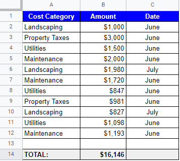
Now, suppose that the analyst wanted to sum all of the Landscaping expenses, but only if they were incurred in July. Using the syntax above, the formula could be written like this:
=SUMIFS(B2:B12,A2:A12,”Landscaping”,C2:C12,”July”)
To understand each of these arguments, it helps to break them down individually:
- Sum Range: The sum range is B2:B12, which represents the dollar amounts to sum.
- Criteria Range 1: The analyst wants to sum the expenses for landscaping, so the first criteria range is A2:A12, which is where the category descriptions are listed.
- Criteria 1: Again, the analyst wants to sum the expenses for landscaping, so their first criteria is “Landscaping.” Remember, it must be in quotes since it is text.
- Criteria Range 2: The second criteria is for landscaping expenses, only in July. As such, the second criteria range is C2:C12. This range contains the month in which the expense was incurred.
- Criteria 2: Finally, the analyst needs to specify that they are only looking for landscaping expenses incurred in July. So, the second criteria is “July.” Again, it must be in quotes.
The result of this formula is $2,807. For additional information on the SUMIFS function, head to the official Microsoft Excel support page, which can be found here.
SUMPRODUCT
The SUMPRODUCT function allows a user to sum and multiply two ranges of values at the same time. In real estate financial models, there is one scenario in which this is particularly useful, the rent roll. The syntax for the SUMPRODUCT function is:
Syntax: =SUMPRODUCT(array1, [array2], [array3], …)
To illustrate how this works, consider the following basic rent roll.
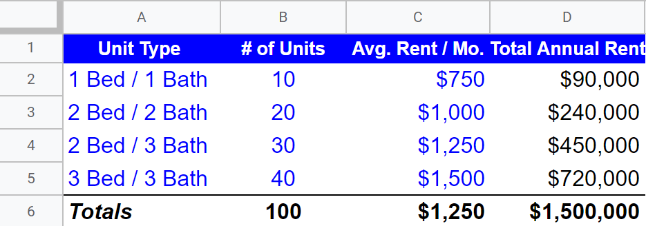
Suppose that the analyst needs to calculate the total annual rental income from this rent roll. There are multiple ways this can be done, but the quickest and easiest is to use the SUMPRODUCT function. The “arrays” represent the columns of data to be summed and multiplied. Column B is the number of units and column C is the monthly rent. So, the total annual rental income is calculated by summing and multiplying these two columns, then multiplying the result by 12. The formula looks like this:
Annual Income = SUMPRODUCT (B2:B5,C2:C5)*12
Writing the formula this way allows the analyst to calculate the total at once versus having to do it over multiple steps, with multiple formulas. To learn more about the SUMPRODUCT function, visit the Microsoft Excel support page, here.
Summary & Conclusion
SUMIF is a conditional Microsoft Excel function that allows users to sum a range of values, but only if they meet certain criteria. It is particularly useful when performing commercial real estate investment and cash flow analysis.
The syntax used to write the formula is “SUMIF(range, criteria, [sum_range])” where the range is the cells that contain the criteria, the criteria is the condition under which values should be summed, and the sum range is the values that should be summed, but only if this range is different than the criteria range.
There are two useful variations of the SUMIF function that are also useful in a real estate finance context. First is the SUMIFS function, which allows a user to sum a range of values based on multiple criteria, and the SUMPRODUCT function which allows a user to sum and multiply a range of values at the same time.